Reviewing Karpathy’s "The Unreasonable Effectiveness of RNNs"

Overview

As the title suggests, this post presents a genuinely shocking result: recurrent neural networks can do far more than one would expect from such a simple formulation.

Training Over Programs

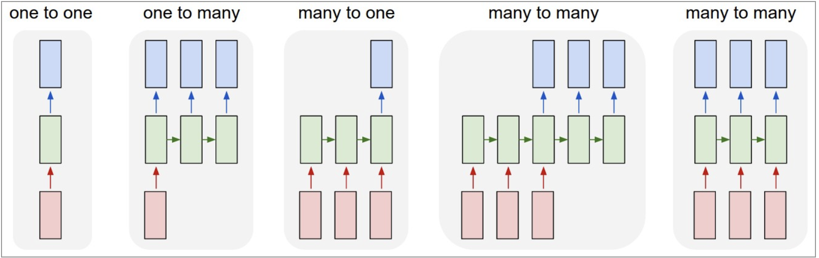
What makes recurrent networks exciting is not merely that they work on sequences, but how they work on them. Unlike vanilla neural networks that map fixed-size inputs to fixed-size outputs in a fixed number of computation steps, RNNs operate over sequences of vectors. It combines the current input with an internal state through a fixed (but learned) transition function, producing a new state at every step. The same transformation is applied repeatedly, allowing the model to naturally handle variable-length inputs, outputs, or both.

Training Recurrent nets is optimization over programs

This flexibility immediately enables a wide range of problem settings: sequence-to-one, one-to-sequence, and sequence-to-sequence mappings all fall out of the same framework. The model is no longer constrained by input size or output length, but instead by how long we choose to unroll it.

More interestingly, Karpathy points out that even when the input and output are fixed-size vectors, recurrent networks remain useful. By processing fixed data sequentially, RNNs effectively turn static inputs into a temporal process. In this view, the network is not learning a single transformation, but a stateful procedure—a small program that updates its internal state step by step.

This perspective reframes recurrent networks as something fundamentally different from feedforward models: rather than learning a static function, they learn how to operate over data through time.

Understanding Vanilla RNNs

A Recurrent Neural Network (RNN) is designed to handle sequential data by maintaining a “memory” of previous inputs.

The Architecture Diagram

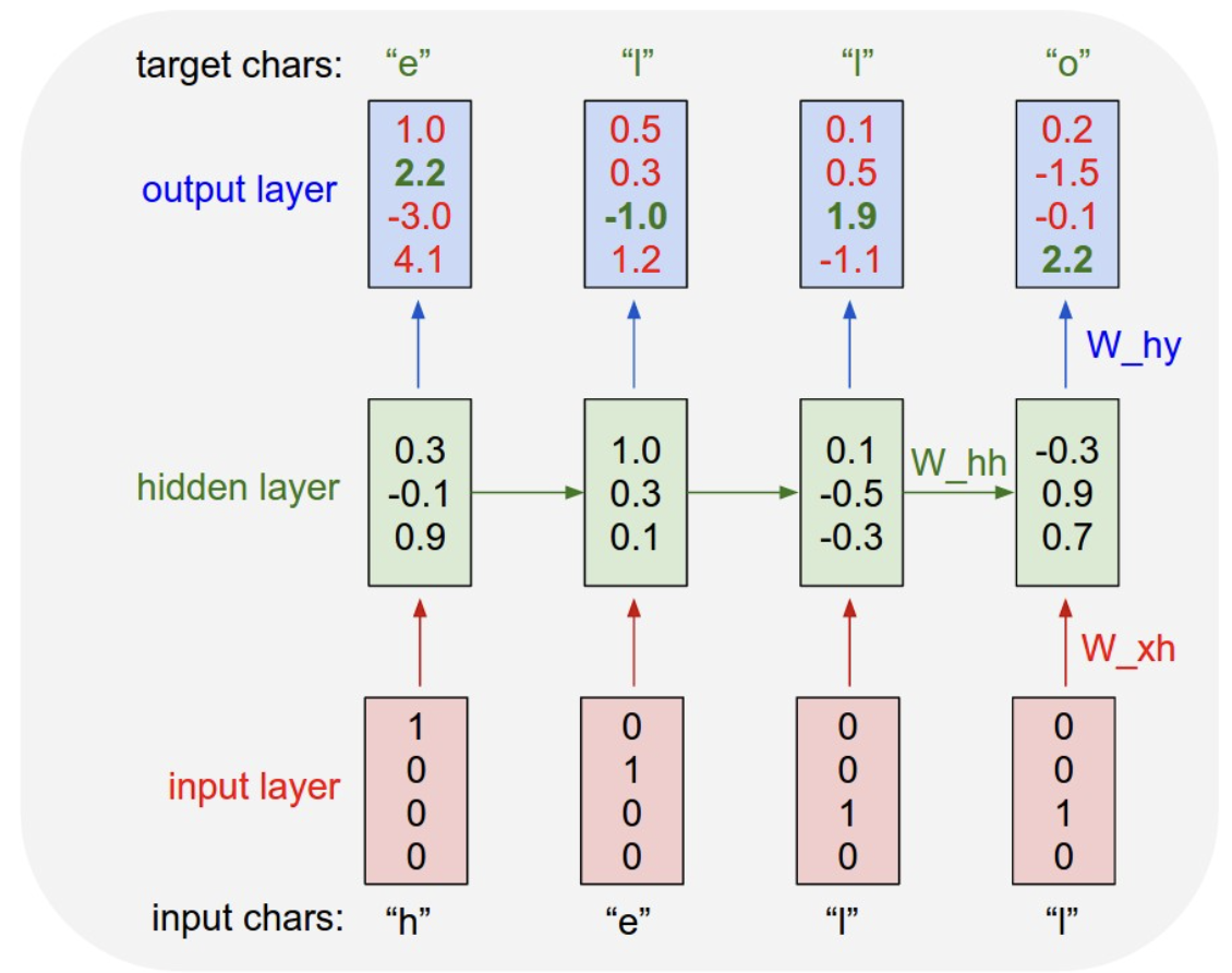
The diagram illustrates an RNN processing the sequence to predict the word “hello”:

Input Characters: “h” $\rightarrow$ “e” $\rightarrow$ “l” $\rightarrow$ “l”
Target Characters: “e” $\rightarrow$ “l” $\rightarrow$ “l” $\rightarrow$ “o”
Input Layer: Uses one-hot encoding (e.g., $[1, 0, 0, 0]^T$ ).
Hidden Layer: A process where state is passed horizontally across time steps.
Output Layer: Produces scores (logits) for the next character prediction.

The Linear Map

The Input-to Hidden Mapping

To move from the input layer to the hidden layer, we need a linear transformation. If we define:

$x \in \mathbb{R}^{input\_{size}\times 1}$ (The input vector)
$h_t \in \mathbb{R}^{hidden\_size\times 1}$ (The hidden state at time $t$ ) The operation follows the shape:

$(\text{hidden\_size} \times \text{input\_size}) \cdot (\text{input\_size} \times 1) = h_t$

Therefore, the weight matrix $W_{xh}$ exists in the space:

$W_{xh} \in \mathbb{R}^{(\text{hidden\_space} \times \text{input\_size})}$

The Recurrent Step (Hidden-to-Hidden)

To maintain continuity, the previous hidden state $h_{t-1}$ is multiplied by the recurrent weight $W_{hh}$ . if we define:

Previous hidden state ( $h_{t-1}$ ): $\mathbb{R}^{hidden\_size \times 1}$
Recurrent weight ( $W_{hh}$ ): $\mathbb{R}^{hidden\_size \times hidden\_size}$ Therefore:

$(hidden\_size \times hidden\_size) \cdot (hidden\_size \times 1) = (hidden\_size \times 1)$

The Hidden-to-Output Mapping

Finally, the current hidden state $h_t$ is mapped to the output space (e.g., for character prediction).

Hidden state ( $h_t$ ): $\mathbb{R}^{hidden\_size \times 1}$
Output weight ( $W_{hy}$ ): $\mathbb{R}^{output\_size \times hidden\_size}$

We have:

$y_t = (output\_size \times hidden\_size) \cdot (hidden\_size \times 1) = (output\_size \times 1)$

While $input\_size$ and $output\_size$ often both equal the vocabulary size $V$ in character-level models, they are independent parameters. The Hidden Size, however, is a hyperparameter we choose to determine the capacity of the model’s memory.”

Why do we need $W_{hh}$ ?

Notice that we need $W_{hh}$ to move horizontally across the network. This is what makes a “Recurrent” Neural Network recurrent.

The “Why”: The network needs context to distinguish between identical inputs at different positions. For example, in the word “hello”:

The first time the character “l” is input, the target is “l”.
The second time the character “l” is input, the target is “o”.

Without the horizontal hidden state ( $W_{hh}$ ), the network would have no way of knowing which “l” it is currently processing.

The RNN Mechanism

An RNN maps an input vector $x$ to an output vector $y$ . Crucially, the output values are influenced not only by the current input being fed, but the entire history of inputs processed so far.

Core Model Equations

For time t:

Input:

$x \in \mathbb{R}^{input\_{size}\times 1}$ (one hot encoding).

Hidden State

The hidden state is updated using a $tanh$ activation function, which squashes the activations to the range $[-1, 1]$ :

$h_t = \tanh(W_{hh} h_{t-1} + W_{xh} x_{t)}+ b_{h}$

In practice, we often have a bias vector.

Output:

$y_{t} = W_{hy}h_{t} + b_{y}$

Wrap up in softmax( cross-entropy loss) $p_{t} = softmax(y_{t})$

In code:

class VanillaRNN:
	# skip weight initializations.
	def rnn_step(x_t, h_prev, params): 
		""" 
		Vanilla RNN forward pass
		x_t: (input_size, 1) 
		h_prev: (hidden_size, 1) 
		""" 
		# update hidden state
		h_t = np.tanh(np.dot(W_hh, h_prev) + np.dot(W_xh, x_t) + b_h) 
		# compute output: 
		y_t = np.dot(W_hy, h_t) + b_y 
		# Softmax 
		p_t = np.exp(y_t) / np.sum(np.exp(y_t)) 
		return h_t, p_t

A Note on Backpropagation Through Time (BPTT)

Loss Function and Backpropagation Through Time (BPTT)

Once the forward pass generates probabilities $p_t$ , we need to measure how well the model performed and update the weights.

Cross-Entropy Loss

For RNNs, the total loss is the sum of the losses at each time step. We use Cross-Entropy Loss, which penalizes the model based on the negative log-probability of the correct character.

$L = \sum_{t} -\log p_t(y_t)$

The Gradient Flow: BPTT

Because weights ( $W_{xh}, W_{hh}, W_{hy}$ ) are shared across all time steps, we use Backpropagation Through Time (BPTT). We iterate backward from the last time step to the first, accumulating gradients.

A critical step in training RNNs is Gradient Clipping. Since we multiply gradients over many time steps, they can “explode.” Clipping forces the gradients to stay within a reasonable range (e.g., $[-5, 5]$ ).

def loss(ps, targets):
    """
    ps: list of probability vectors for each time step
    targets: list of ground-truth indices for each time step
    """
    total_loss = 0
    for t in range(len(targets)):
        # -log of the probability assigned to the correct class
        total_loss += -np.log(ps[t][targets[t], 0])
    return total_loss

def backward(self, xs, hs, ps, targets):
    """
    Backpropagation Through Time (BPTT)
    xs: inputs, hs: hidden states, ps: probabilities
    """
    dWxh, dWhh, dWhy = np.zeros_like(self.W_xh), np.zeros_like(self.W_hh), np.zeros_like(self.W_hy)
    dbh, dby = np.zeros_like(self.bh), np.zeros_like(self.by)
    
    # Gradient of the hidden state from the "future"
    dhnext = np.zeros_like(hs[0])

    # Iterate backwards through the sequence
    for t in reversed(range(len(targets))):
        # 1. Gradient of Loss w.r.t Output (dy = p_t - y_true)
        dy = np.copy(ps[t])
        dy[targets[t]] -= 1 
        
        # 2. Gradients for Output Layer
        dWhy += np.dot(dy, hs[t].T)
        dby += dy
        
        # 3. Gradients for Hidden State (flowing back from output and next state)
        dh = np.dot(self.W_hy.T, dy) + dhnext
        
        # 4. Backprop through tanh: derivative is (1 - h^2)
        dhraw = (1 - hs[t] * hs[t]) * dh 
        
        # 5. Accumulate gradients for weights and biases
        dbh += dhraw
        dWxh += np.dot(dhraw, xs[t].T)
        dWhh += np.dot(dhraw, hs[t-1].T)
        
        # 6. Pass the gradient to the previous time step
        dhnext = np.dot(self.W_hh.T, dhraw)

    # Gradient Clipping to prevent Exploding Gradients
    for dparam in [dWxh, dWhh, dWhy, dbh, dby]:
        np.clip(dparam, -5, 5, out=dparam)

    return dWxh, dWhh, dWhy, dbh, dby

Why this was a “wow” moment for me

What truly surprised me was not the RNN formulation itself, but the examples Karpathy showed.

By training on raw character sequences, the model could appear to understand highly structured domains such as mathematics and LaTeX. Of course, it does not actually understand proofs or mathematical meaning, but it can convincingly pretend to operate within those systems.

Seeing an RNN generate LaTeX that almost compiles, respects environments, and follows familiar mathematical notation was a turning point for me. It suggested that the usefulness of recurrent models goes far beyond natural language: any domain with strong syntactic regularities can be modeled as a sequence.

This was the moment I realized that the power of RNNs is not tied to semantics, but to structure. As long as a task can be expressed as a sequence of symbols with consistent constraints, a recurrent model can learn to behave as if it “understands” the domain—even when it clearly does not.

Reference:

https://karpathy.github.io/2015/05/21/rnn-effectiveness/ https://gist.github.com/karpathy/d4dee566867f8291f086 https://github.com/pageman/sutskever-30-implementations?tab=readme-ov-file