Autoencoders

Introduction

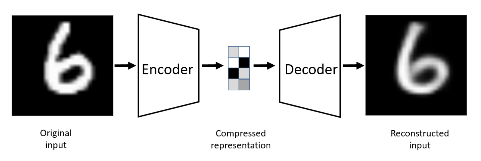
An autoencoder is a neural network designed to learn a compressed, informative representation of input data. It does this by mapping the input x into a lower-dimensional latent code z (the latent space) using an encoder, and then mapping z back to a reconstruction $\hat{x}$ using a decoder, with the goal that $\hat{x}$ is as close as possible to x. A vanilla autoencoder is a deterministic latent-space model: for a fixed input x, the encoder always produces the same z, and no explicit probability distribution is involved.

Note

Mathematically,

Let dataset $\mathcal{D}=\{x_{n}\}^N_{{n=1}}$ where $x_{n}\in \mathcal{X}$.

$Enc_{\theta}:\mathcal{X}\mapsto z$ be a neural net with parameter $\theta$, where it learns to encode x. $Dec_{\phi}:z\mapsto \mathcal{X}$ be a neural net with parameter $\phi$, where it learns to reconstruct x from its encoding.

The problem can then phrase to be

$\mathbb{E}_{x \sim p(x)}[\Delta(x, B(A(x)))] \;\approx\; \frac{1}{N}\sum_{n=1}^N \frac12 \|x_n - \text{Dec}_\phi(\text{Enc}_\theta(x_n))\|^2$.

A autoencoder model use unsupervised learning to discover the latent variables of the input data(not directly observable but fundamentally inform the way data is distributed) then to reconstruct their own input data that has the same dimensions.

Types

1. Vanilla Autoencoders: Basic autoencoders that efficiently encode and decode data

2. Denoising Autoencoders: Improved robustness to noise and irrelevant information

3. Sparse Autoencoders: Learn more compact and efficient data representations

4. Contractive Autoencoders: Generate representations less sensitive to minor data variations

5. Variational Autoencoders: Generate new data points that resemble in some form the training data.

In essential, auto-encoders are designed to learn a lower-dimensional representation for a higher-dimensional data.

Applications include: 1. dimensionality reduction; 2. Feature extraction; 3. Image Denoising; 4. Image Compression; 5. Image Search; 6. Anomaly Detection; 7. Missing value imputation

Architecture:

The autoencoder maps the space of decoded message $X$ to the space of encoded message $Z$. In most cases, both $X$ and $Z$ are Euclidean spaces($X=R^m$ and $Z=R^n$ for some $m,n$)

We describe the autoencoder algorithm in two parts:

1. encoder function: a parametrized family of encoder functions $f_{\theta}$ , parametrized by $\theta$, that maps an input $x\in X$ to a code $h\in Z$

2. decoder function: a parametrized family of encoder functions $g_{\phi}$ , parametrized by $\phi$, that maps $h\in Z$ to $x'\in X$

$g_{\phi}(h)= x'$

The decoder is designed to produce a reconstruction $X'$ of the input $X$.

Both the encoder and decoder function is defined as MLPs. A one-layer MLP encoder is in the form

3. The Loss Function

The loss function penalizes $X'=g_{\phi}(h)=g_{\phi}(f_{\theta}(X))$ for being dissimilar from X.

In the continuous setting, let $\mu$ be a reference probability distribution on X and $d: X \times X \rightarrow R$ be a distance function. Thus,

$L(\theta,\phi):E_{x\sim \mu_{ref}}[d(x,g_{\phi}(f_{\theta}(x)))]$

The optimal autoencoder is defined by the optimization problem

In practical, $\mu_{ref}$ is empirical distribution given by a dataset $\{X_{1,\dots,X_{N}}\} \subset X$

So is the Dirac measure $\mu_{ref}=\frac{1}{n}\sum^n_{i=1}\_{x_{i}}$

The distance function is typically chosen to be the square $L^2$ loss

$d(x,x')=||x-x'||^2_{2}$

Hence the optimal autoencoder search becomes:

$L(\theta,\phi)=\frac{1}{n}\sum^n_{i=1}||X_{i}-g_{\phi}(f_{\theta}(X_{i}))||^2_{2}$

Autoencoders are designed to be unable to learn the identity functions. It can learn useful properties of the data by prioritize which aspect of input should be copied.

Training

1. Number of nodes per layer : the standard autoencoder architecture we had above is called stacked autoencoder

2. Loss function : usual choices are MSE or crossentropy

3. Trained via backpropagation and mini-batch gradient descent

Interpretation:

An autoencoder is optimized to perform as close to perfect reconstruction as possible. In many applications, the goal is to create a reduced set of codings that represents the inputs.

An autoencoder whose internal representation has a smaller dimensionality than the input data is an undercomplete autoencoder.

Remark: When the autoencoder uses only linear activation functions and the loss function is MSE, then the autoencoder learns to span the same subspace as Principal Component Analysis (PCA)

When nonlinear activation functions are used, autoencoders provide nonlinear generalizations of PCA

Bottleneck is to prevent the autoencoder from overfitting to its training data. Otherwise, it tends toward learning the identity function

Thus:

Limitation:

1. when hidden code $h$ has the same dimension as input $x$

2. Even in the case of an undercomplete autoencoder, the capacity of encoder/decoder is too high(processing large or complex data inputs)

3. Overcomplete case: hidden code $h$ has dimension greater than input $X$

Regularization

By introducing regularization, we prevent autoencoder from learning the identity function.

1. Denoising Autoencoder

2. Sparse Autoencoder

3. Contractive Autoencoder

Denoisng autoencoder

Objective:

1. try to encode the inputs the preserve the essential signals;

2. try to undo the effects of a corruption process stochastically applied to the inputs of the autoencoder.

We train the autoencoder from a corrupted copy of the input.

corruption typically follows: additive Gaussian noise; masking noise; salt-and-pepper noise

DAE is associated to a different loss function as compared to a vanilla autoencoder

Loss function:

Letting the noise process be defined by a probability distribution $\mu_{T}$ over functions$T: X\mapsto X$

Sparse Autoencoders

Objective

designed to pull out the*** most influential feature*** representations of the input data by using a sparsity constraint such that only a fraction of the nodes would have nonzero values.

A penalty directly proportional to the number of neurons activated is applied to the loss function

Sparse autoencoders may include more (rather than fewer) hidden units than inputs as the code$f_{\theta}(X)$ is close to zero in most entries.

To enforce sparsity

1. k-sparse

Suppose the encoder produces a latent vector:

$(x_1, x_2, \dots, x_n)$

• Compute the absolute values: |x_1|, |x_2|, \dots, |x_n|.

• Rank them from largest to smallest.

• Keep only the top-k largest values (by magnitude).

• Set all the other entries to zero.

$f_{k}(x_1, x_2, \dots, x_{n)}= (x_{1}b_{1},\dots, x_{n}b_{n})$

Where $b_{i}=1$ if $|x_{i}|$ ranks in the top k, and 0 otherwise.

Backpropagating through $f_{k}$: set gradient to $0$ for $b_{i}=0$ entries and keep gradient for $b_{i}=1$ entries.

The hidden nodes in bright yellow are activated.

2. Add a sparsity regularization loss

Optimize for:

$\min_{\theta, \phi} \; L(\theta, \phi) + \lambda L_{\text{sparsity}}(\theta, \phi)$

For each hidden layer k, we measure average activation:

$\rho_k(x) = \frac{1}{n} \sum_{i=1}^n a_{k,i}(x)$

• $a_{k,i}(x)$: activation of neuron i in layer k given input x.

• $\rho_k(x)$: average fraction of neurons active in that layer for input x.

We use a function $s(\hat{\rho}_k, \rho_k(x))$ to measure how far the actual sparsity $\rho_k(x)$ is from the desired sparsity $\hat{\rho}_k.$

Where

$L_{\text{sparsity}}(\theta, \phi) = \mathbb{E}_{x \sim \mu_X} \left[ \sum_{k=1}^K w_k \, s(\hat{\rho}_k, \rho_k(x))\right]$

Choices for the function s: Kullback-leibler divergence; L1 loss; L2 loss

Contractive Audoencoder:

Adds a contractive regularization loss the the standard autoencoder loss that penalizes the network for changing the output in response to insufficiently large changes in the input.

$\min_{\theta, \phi} \; L(\theta, \phi) + \lambda L_{\text{contractive}}(\theta, \phi)$

The encoder is a function $f_\theta(x)$ that maps input x to latent code z.

The Jacobian matrix of $f_\theta$ wrt x is:

$J_{f_\theta}(x) = \frac{\partial f_\theta(x)}{\partial x}$

Each entry shows how much a latent dimension changes when you nudge one input dimension.

If this Jacobian has small values → the latent code doesn’t change much when inputs vary slightly.

We measure the “size” of the Jacobian using the Frobenius norm:

$\|J_{f_\theta}(x)\|_{F}^2 = \sum{i,j} \left(\frac{\partial f_{\theta,i}(x)}{\partial x_j}\right)^2$

The contractive regularization loss is:

$L_{\text{contractive}}(\theta, \phi) = \mathbb{E}{x \sim \mu{\text{ref}}} \, \| \nabla_x f_\theta(x) \|_F^2$

They note that for small perturbations $\delta x$:

$\|f_\theta(x + \delta x) - f_\theta(x)\|2 \;\leq\; \|\nabla_x f\theta(x)\|_F \cdot \|\delta x\|_2$

So:

• If $|\nabla_x f_\theta(x)\|_F$ is small, then even if you perturb the input slightly ($\delta x$), the change in the code is small.

• This makes the latent space stable and contractive around each data point.

Manifold Learning

Manifold Hypothesis

Data concentrates around a low-dimensional manifold

Some ML algorithm have unusual behavior if given an input that is off of the manifold.

Example:

Setting:

An image of size m \times n pixels can be written as a vector in $\mathbb{R}^N$, where $N = m \times n.$

Let’s say A 100×100 image → $N = 10,000$.

So each image is one point in a huge-dimensional space.

Restriction:

Not All Pixel Combinations Make Sense

Most points in this huge space do not look like valid images of Einstein.

Valid Einstein images only occupy a very tiny subset of this space.

The manifold hypothesis says:

• Even though Einstein images live in a high-dimensional space (N),

• They actually lie on a low-dimensional manifold within it.

Definition of Manifold

An n-dimensional manifold is a topological space M for which every point $x \in M$ has a neighborhood homeomorphic to Euclidean space $\mathbb{R}^n$.

Homeomorphism in topology is also called a continuous transformation

One-to-one correspondence in two geometric figures or topological spaces that is continuous in both directions

Homomorphism in algebra

The most important functions between two groups are those that preserve group operations, and they are called homomorphisms.

A function $f: G \to H$ between two groups is a homomorphism when

$f(xy) = f(x)f(y) \quad \text{for all } x,y \in G$

A manifold has a dimension:

2-D manifold is a surface

1-D manifold is a curve

0-D manifold is a point

Manifold hypothesis = the decoder assumption of autoencoders/VAEs.

In the observed $M$-dimensional input space, the data is distributed on an $M_{h}$-dimensional manifold where $M_h < M$

There exists a smooth function $g^{\text{gen}}$ such that:

$\mathbf{x} = g^{\text{gen}}(\mathbf{h})$

$\mathbf{h}$: hidden (intrinsic) coordinates on the manifold.

$g^{\text{gen}}$: the generative process that maps hidden factors into observed data.

$\mathbf{x}:$ the actual observed data point in high dimension.

tangent = local linear approximation of the manifold

At a point x on a d-dimensional manifold, the tangent plane is given by d basis vectors that span the local directions of variation allowed on the manifold

• On a curve (1D manifold): the tangent line tells you the local direction of movement at a point. $y \approx f(x^0) + f’(x^0)(x - x^0)$

• On a surface (2D manifold): the tangent plane tells you the set of directions you can move infinitesimally while staying on the surface

Autoencoder performs trade-off between two forces

1. learns representation $h$ of training example x such that x can be recovered through a decoder

2. satisfies the regularization penalty

Together they force the hidden representation to capture information about the data generating distribution

The encoder learns to ignore noise (off-manifold directions) and focus only on meaningful changes (on-manifold tangent directions). That’s why autoencoders can capture the true low-dimensional structure of data.

https://cedar.buffalo.edu/~srihari/CSE676/14.3%20Learning%20Manifolds.pdf

Variational autoencoder

VAEs are trained to learn The probability distribution that models the input-data and not the function that maps the input and the output.

Difference between VAEs and other types of autoencoder:

VAEs learn continuous latent variable models

Most autoencoder learn discrete latent space models.

In a standard autoencoder, the encoder outputs a fixed latent vector:

$z = f_\theta(x)$

This z is just a point in latent space (a deterministic code). There is no uncertainty — each input maps to one exact representation.

In a VAE, the encoder doesn’t output a point but a distribution over latent codes:

$q_\phi(z|x) = \mathcal{N}(z; \mu_\phi(x), \sigma^2_\phi(x))$

This makes z a continuous random variable sampled from a smooth space.

Objective

Given an input dataset x characterized by an unknown probability function $P(x)$ and a multivariate latent encoding vector z, the objective is to model the data as a distribution $p_{\theta}(x)$ with $\theta$ defined as the set of the network parameters so that

$p_{\theta}=\int_{z}p_{\theta}(x,z)dz$

VAE is generative AI models as it learns the latent distribution

VAEs can sample points from the latent distribution and feed them to the decoder to generate new samples that resemble the original training data

Application include: image generation and synthesis; Representation learning›

Loss function: two components:

1. The reconstruction loss: (MSE/ cross-entropy) Measures how different the reconstructed data are from the original data

2. KL-divergence: tries to regularize the process and keep the reconstructed data as diverse as possible.

$L_{\theta, \phi}(x) = - \mathbb{E}_{z \sim q_\phi} \big[ \ln p_\theta(x|z) \big] + D_{KL}\!\left(q_\phi(z|x) \,\|\, p_\theta(z)\right)$

Mathematical formulation

We want to model the data distribution $p_\theta(x)$, so we can:

• Learn representations of data (encoding).

• Generate new realistic samples (decoding).

Formally, we maximize the log-likelihood:

$\max_\theta \ \ln p_\theta(x)$

We introduce a latent variable $z$ that explains the data $x$.

$p_\theta(x) = \int p_\theta(x, z) \, dz$

By the chain rule（factorization of a joint distribution $p_\theta(x, z) = p_\theta(x|z) \, p_\theta(z)$):

$p_\theta(x) = \int p_\theta(x|z) \, p_\theta(z) \, dz$

• $p_\theta(z)$: prior (assumed to be $\mathcal{N}(0, I))$.

• $p_\theta(x|z)$: likelihood / decoder (how data is generated from latent $z$).

• $p_\theta(z|x)$: posterior / encoder (how latent variables are distributed given data).

The posterior:

$p_\theta(z|x) = \frac{p_\theta(x|z)p_\theta(z)}{p_\theta(x)}$

is usually intractable (the denominator requires integrating over all $z$).

$D_{KL}\!\big(q_\phi(z|x) \,\|\, p_\theta(z|x)\big)$

Gaussian Assumption

Prior:

$p_\theta(z) \sim \mathcal{N}(0, I)$

Decoder:

$p_\theta(x|z) \sim \mathcal{N}(f_\theta(z), cI)$

Where $p_\theta(x|z)$ is a Gaussian distribution whose mean is defined by a deterministic function $f\in F$ of the variable of z and covariance is a positive constant $c$ that multiplies $I$

Encoder:

$q_\phi(z|x) \sim \mathcal{N}(g_\phi(x), h_\phi(x))$

Approximate using variational inference

To set a parametrized family of distribution - for example the family of Gaussians, whose parameters are the mean and the covariance - and to look for the best approximation of our target distribution among this family.

This is found computationally by gradient descent over the parameters that describe the family.

We approximate the posterior$p_\theta(z|x)$ with a variational distribution:

$q_\phi(z|x) \approx p_\theta(z|x)$

• $q_\phi(z|x)$ is parameterized by the encoder neural network (mean + variance of a Gaussian).

$q_{\phi(z|x)}= N(g_{[\phi]}(x),h_{\phi}(x))$

to the parametrized families of functions G and H.

• The quality of approximation is measured by KL divergence:

Evidence Lower Bound (ELBO)

We derive a lower bound on $\ln p_\theta(x)$:

$L_{\theta, \phi}(x) := \mathbb{E}_{z \sim q_\phi(\cdot|x)} \left[ \ln \frac{p_\theta(x, z)}{q_\phi(z|x)} \right] = \ln p_\theta(x) - D_{KL}\!\left(q_\phi(\cdot|x) \,\|\, p_\theta(\cdot|x)\right)$

Maximizing the ELBO

$\theta^*, \, \phi^* = argmax_{\theta, \phi} \, L_{\theta, \phi}(x)$

Is equivalent to simultaneously maximizing $ln p_\theta(x)$ and minimizing $D_{KL}$

Rewrite:

$L_{\theta, \phi}(x)=\mathbb{E}_{z \sim q_\phi(\cdot|x)} \big[ \ln p_\theta(x|z) \big]-D_{KL}(q_\phi(\cdot|x) \,\|\, p_\theta(\cdot))$

Under the assumption that $x\sim N(D_{\theta}(z),I)$, that is, we model the distribution of x on z to be a Gaussian distribution centered on $D_{\theta}(z)$

Then:

$\ln p_\theta(x|z) \propto -\tfrac{1}{2}\|x - D_\theta(z)\|^2$

Gaussian PDF:

$p(x) = \frac{1}{(2\pi\sigma^2)^{d/2}} \exp\!\left(-\frac{1}{2\sigma^2} \|x - \mu\|^2\right)$>Take log:

$\ln p(x) = -\frac{d}{2}\ln(2\pi\sigma^2) - \frac{1}{2\sigma^2}\|x - \mu\|^2$>Assume unit variance ($\sigma^2 = 1$):

$\ln p(x) = -\frac{d}{2}\ln(2\pi) - \tfrac{1}{2}\|x - \mu\|^2$>Drop constants (they don’t affect optimization):$\ln p(x) \propto -\tfrac{1}{2}\|x - \mu\|^2$ >In VAE:$\mu = D_\theta(z)$, so:

$\ln p_\theta(x|z) \propto -\tfrac{1}{2}\|x - D_\theta(z)\|^2$

We assume:

Encoder:$q_\phi(z|x) = \mathcal{N}(E_\phi(x), \, \sigma_\phi(x)^2 I)$

Prior:

$p(z) = \mathcal{N}(0, I)$

And: The KL between two Gaussians has a closed form:

$D_{KL}(\mathcal{N}(\mu, \sigma^2 I) \,\|\, \mathcal{N}(0, I)) = \tfrac{1}{2} \left( \|\mu\|^2 + N\sigma^2 - 2N \ln \sigma - N \right)$

Thus:

$L_{\theta,\phi}(x) = -\tfrac{1}{2}\, \mathbb{E}{z \sim q\phi(z|x)} \|x - D_\theta(z)\|^2 • \tfrac{1}{2}\Big(N\sigma_\phi(x)^2 + \|E_\phi(x)\|^2 - 2N\ln\sigma_\phi(x)\Big) + \text{Const}$

Where $N$ is the dimension of z.

Reparameterization trick:

Problem: Directly sampling $z \sim \mathcal{N}(\mu_\phi(x), \sigma_\phi(x)^2)$ is random → no gradients can flow back to $\mu_\phi(x), \sigma_\phi(x)$.

Trick: Write sampling as

$z = \mu_\phi(x) + \sigma_\phi(x) \odot \epsilon, \quad \epsilon \sim \mathcal{N}(0, I)$Why it works:

Randomness comes only from$\epsilon$ (fixed distribution).

$\mu_\phi(x) \text{ and } \sigma_\phi(x)$ are differentiable → gradients can flow.

Result: Encoder and decoder can be trained end-to-end with backpropagation

VAEs Code Tutorial https://www.codecademy.com/article/variational-autoencoder-tutorial-vaes-explained

Step1 Setting up the VAE environment

import torch

import torch.nn as nn

import torch.nn.functional as F

from torchvision import datasets, transforms

from torch.utils.data import DataLoader

import matplotlib.pyplot as plt

  

device = torch.device("cuda" if torch.cuda.is_available() else "cpu")

  

# Load MNIST dataset

transform = transforms.ToTensor()

train_dataset = datasets.MNIST(

root="./data",

train=True,

transform=transform,

download=True,

)

train_loader = DataLoader(

dataset=train_dataset,

batch_size=128,

shuffle=True,

)

  

Step 2 Building the VAE model architecture

(Encoder)

  

class Encoder(nn.Module):

def __init__(self, input_dim: int = 784, hidden_dim: int = 400, latent_dim: int = 20):

super().__init__()

self.fc1 = nn.Linear(input_dim, hidden_dim)

self.fc_mu = nn.Linear(hidden_dim, latent_dim)

self.fc_logvar = nn.Linear(hidden_dim, latent_dim)

  

def forward(self, x: torch.Tensor) -> tuple[torch.Tensor, torch.Tensor]:

h = torch.relu(self.fc1(x))

mu = self.fc_mu(h)

logvar = self.fc_logvar(h)

return mu, logvar

  

(Decoder)

  

class Decoder(nn.Module):

def __init__(self, latent_dim: int = 20, hidden_dim: int = 400, output_dim: int = 784):

super().__init__()

self.fc1 = nn.Linear(latent_dim, hidden_dim)

self.fc2 = nn.Linear(hidden_dim, output_dim)

  

def forward(self, z: torch.Tensor) -> torch.Tensor:

h = torch.relu(self.fc1(z))

return torch.sigmoid(self.fc2(h))

  

Creating the main VAE class

  

class VAE(nn.Module):

def __init__(self, input_dim: int = 784, hidden_dim: int = 400, latent_dim: int = 20):

super().__init__()

self.encoder = Encoder(input_dim, hidden_dim, latent_dim)

self.decoder = Decoder(latent_dim, hidden_dim, input_dim)

  

def reparameterize(self, mu: torch.Tensor, logvar: torch.Tensor) -> torch.Tensor:

std = torch.exp(0.5 * logvar)

eps = torch.randn_like(std)

return mu + eps * std

  

def decode(self, z: torch.Tensor) -> torch.Tensor:

return self.decoder(z)

  

def forward(self, x: torch.Tensor) -> tuple[torch.Tensor, torch.Tensor, torch.Tensor]:

mu, logvar = self.encoder(x)

z = self.reparameterize(mu, logvar)

recon_x = self.decoder(z)

return recon_x, mu, logvar

  

  

Here we used reparameterization tricks as sampling directly from a distribution breaks backpropogation. we sample ε ~ N(0,1) and compute z = μ + σ * ε instead.

Step 3 Defining the loss function

  

def loss_function(recon_x: torch.Tensor, x: torch.Tensor, mu: torch.Tensor, logvar: torch.Tensor) -> torch.Tensor:

# Reconstruction loss (binary cross entropy)

recon_loss = F.binary_cross_entropy(recon_x, x, reduction="sum")

# KL divergence loss

kl_loss = -0.5 * torch.sum(1 + logvar - mu.pow(2) - logvar.exp())

return recon_loss + kl_loss

  

Step 4 Training the evaluating the VAE

epochs = 10

learning_rate = 1e-3

  

model = VAE().to(device)

optimizer = torch.optim.Adam(model.parameters(), lr=learning_rate)

  

train_losses = []

  

model.train()

for epoch in range(epochs):

total_loss = 0.0

  

for batch_idx, (x, _) in enumerate(train_loader):

x = x.view(-1, 784).to(device) # Flatten images

optimizer.zero_grad()

  

recon_x, mu, logvar = model(x)

loss = loss_function(recon_x, x, mu, logvar)

  

loss.backward()

optimizer.step()

  

total_loss += float(loss.item())

  

avg_loss = total_loss / len(train_loader.dataset)

train_losses.append(avg_loss)

print(f"Epoch {epoch + 1}/{epochs} | Loss: {avg_loss:.4f}")

  

plt.plot(train_losses)

plt.title("VAE Training Loss")

plt.xlabel("Epoch")

plt.ylabel("Loss")

plt.grid(True)

plt.show()

  

  

Step 5: Testing the VAE by generating new samples

  

model.eval()

  

with torch.no_grad():

z = torch.randn(16, 20).to(device) # 16 samples, 20-d latent

generated = model.decode(z).cpu().view(-1, 1, 28, 28)

  

fig, axes = plt.subplots(2, 8, figsize=(12, 4))

for i, ax in enumerate(axes.flat):

ax.imshow(generated[i][0], cmap="gray")

ax.axis("off")

plt.suptitle("Generated Samples from Latent Space")

plt.show()

  

Step 6 Interpolating

  

def interpolate(model: VAE, z_start: torch.Tensor, z_end: torch.Tensor, steps: int = 10) -> torch.Tensor:

ts = torch.linspace(0, 1, steps, device=device).view(-1, 1)

vectors = z_start.to(device) * (1 - ts) + z_end.to(device) * ts # (steps, latent_dim)

  

model.eval()

with torch.no_grad():

samples = model.decode(vectors).cpu()

  

return samples.view(-1, 1, 28, 28)

  

z1 = torch.randn(1, 20)

z2 = torch.randn(1, 20)

  

interpolated_images = interpolate(model, z1, z2, steps=10)

  

fig, axes = plt.subplots(1, 10, figsize=(15, 2))

for i, ax in enumerate(axes.flat):

ax.imshow(interpolated_images[i][0], cmap="gray")

ax.axis("off")

plt.suptitle("Latent Space Interpolation")

plt.show()