Finding the "Invisible": A Topological Approach

The Intuition: What Makes a Data Point “Important”

In high-dimensional data discovery (like finding rare biological lineages), we often hit a wall. Traditional approaches ask: “Where is the model uncertain?” or “Where is the space empty?”

But there is a blind spot. In complex manifolds, rare data often forms thin, branching structures extending into the void. Such as in Biology, cell differentiation is often modeled as a continuous process with branching trajectories in gene expression space.(Rizvi et al., 2017) Standard methods treat these sparse regions as noise or outliers where they fail to see the structure.

This led me to a new hypothesis:

Rare data points are critical “topological anchors” that define the branching structures and connectivity of the underlying manifold

But how do we turn this philosophical idea into an algorithm? We need math.

Bridging the Gap between Points and Manifolds

In machine learning, we rely on the Manifold Hypothesis, which posits that high-dimensional data is not scattered randomly through space but instead resides on a lower-dimensional, continuous surface called a manifold. However, to understand how a manifold structure emerges from discrete data, we must first return to the foundational language of topological spaces.

Definition (Topological Space)

A topological space is a pair $(X, \tau)$, where $X$ is a set and $\tau$ is a collection of subsets of $X$, satisfying:

1. $\emptyset \in \tau$ and $X \in \tau$.
2. Any union of elements of $\tau$ is in $\tau$ (Infinite union).
3. Any finite intersection of elements of $\tau$ is in $\tau$.

And this leads to our important concept of manifold.

Manifold

Definition (Manifold)

Suppose M is a topological space. We say that M is a topological manifold of dimension n or a topological n-manifold if it has the following properties:

1. M is a Hausdorff space
2. M is second-countable: there exists a countable basis for the topology of M .
3. M is locally Euclidean of dimension n: each point of M has a neighborhood that is homeomorphic to an open subset of $R^n$.

While a manifold locally looks like Euclidean space, a purely topological manifold has no geometry. It is like a sheet of rubber—it can be stretched or crumpled as long as it isn’t torn. When embedded in high-dimensional space, it might appear perfectly smooth or infinitely wrinkled(Dey & Wang, 2022)

Smooth Manifold

To make a manifold “useful” for data science, we must upgrade it to a Smooth Manifold by imposing a differential structure:

While a topological manifold is merely continuous (you can stretch it), a smooth manifold allows us to do calculus. This is achieved by requiring the “transition maps” between our local coordinate systems to be not just continuous, but differentiable (smooth, or $C^\infty$).

• The Power of the Tangent Space: This smoothness is what allows us to rigorously define the Tangent Space ($T_xM$) at any point $x$. The tangent space is a local vector space that linearizes the manifold at that point—essentially, the “flat plane” touching the curved surface.

• Why it Matters for AI: Gradients live in the tangent space. Without a smooth differential structure, the concept of a “direction of steepest descent” is ill-defined. You couldn’t use Gradient Descent to train a model, because the manifold wouldn’t have a computable “slope” to slide down.

The Point Cloud: Data in the Wild

Because the manifold is not directly observed, we only have a static list of numbers — like rows in a CSV file. From the perspective of Topological Data Analysis, this raw data is viewed as a point cloud. Formally, a point cloud is a finite set of samples that, in its raw state, carries no inherent geometric or topological structure:

Definition Point Cloud

$P = \{x_1, x_2, \dots, x_n\}$

To make this set suitable for topological analysis, we must equip it with a distance function $d : P \times P \rightarrow \mathbb{R}_{\ge 0}$. This transformation turns $P$ into a finite metric space $(P,d)$, providing the necessary “ruler” to measure relationships between points. We then connect these isolated dots into a coherent “scaffolding” called a Simplicial Complex.

Think of a simplicial complex as a “scaffolding” or a Lego model of the manifold. It is built from simple geometric units called simplices:

• 0-simplex: A point (the data itself).
• 1-simplex: An edge (connecting two points).
• 2-simplex: A triangle (filling the space between three points).

The Nerve Theorem: The Bridge

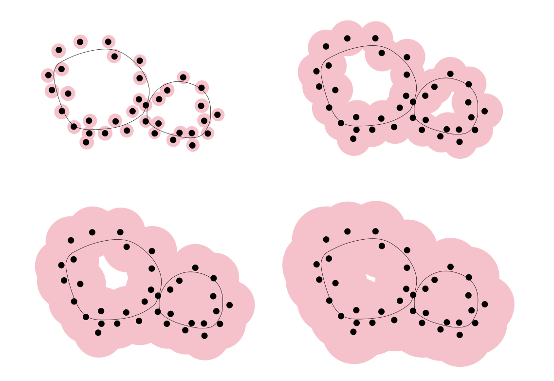
Once a metric is defined, we can grow metric balls around each point. Crucially, it is not the balls themselves that matter, but the pattern of their overlaps. These intersection relationships induce a simplicial complex — specifically, the Čech complex, which is the nerve of this ball covering.

Definition Nerve

Given a collection of sets $\mathcal{U}=\{U_\alpha\}_{\alpha\in A}$, the nerve $N(\mathcal{U})$ is the simplicial complex whose simplices correspond to non-empty intersections:

$$U_{\alpha_0}\cap \cdots \cap U_{\alpha_k} \neq \varnothing.$$

Definition Čech Complex

Let $(M,d)$ be a metric space and $P \subset M$ finite. For $r>0$, the Čech complex $\check{C}_r(P)$ is the nerve of the balls $B(p,r)=\{x\in M \mid d(p,x)\le r\}.$

The theoretical cornerstone of this construction is the Nerve Theorem.

Nerve Theorem

Given a finite cover $\mathcal{U}$ (open or closed) of a metric space $M$,   the underlying space $|N(\mathcal{U})|$ is homotopy equivalent to $M$   if every non-empty intersection $\bigcap_{i=0}^{k} U_{\alpha_i}$ of cover elements is homotopy equivalent to a point, that is, contractible.

Which it states that if the sampling is sufficiently dense and the radius $r$ is chosen appropriately, this simplicial complex is homotopy equivalent to the underlying continuous manifold. In this way, the simplicial complex acts as a bridge, allowing us to recover the hidden manifold structure from discrete data.

The Pragmatic Choice: Čech–Rips Interleaving

While the Nerve Theorem guarantees that the Čech complex is homotopy equivalent to the underlying manifold, calculating multi-way intersections of balls in high-dimensional space is computationally expensive. In practice, we use the Vietoris-Rips complex as a more efficient alternative.

Definition The Rips Complex

For a finite metric space $(P, d)$ and a radius $r > 0$, a simplex $\sigma$ belongs to the complex $\mathbb{V}\mathbb{R}^r(P)$ if and only if $d(p, q) \le 2r$ for every pair of vertices in $\sigma$.

In other words:

• If two points are within $2r$ of each other, we draw an edge.
• If three points are all within $2r$ of each other, we fill in a triangle.

We can justify this substitution through the Čech–Rips Interleaving proposition:

Proposition

Proposition: Interleaving

$\check{C}_r(P) \subseteq VR_r(P) \subseteq \check{C}_{2r}(P)$

Notice that: The interleaving relationship $\check{C}_r(P) \subseteq VR_r(P) \subseteq \check{C}_{2r}(P)$ implies that the Rips complex is “looser” than the Čech complex at the same radius. Because the Rips complex only checks pairwise distances, it can fill in a triangle (a 2-simplex) even if there is no common intersection between all three balls—essentially “overfilling” a hole that the Čech complex would have correctly identified as empty

Filtration (The “Zoom Out” Movie)

But what is the right radius $r$?

• Too small? Everything is disconnected dust.
• Too large? Everything is one giant blob. TDA says: “Don’t choose one. Look at all of them.” We gradually increase the radius from 0 to $\infty$. This dynamic process of growing connections is called a Filtration.

Mathematically, we can view this as looking at the sublevel sets of a distance function (the union of balls growing). However, effectively computing these continuous shapes is difficult.

Computationally, we simulate this “Zoom Out” movie using the discrete Rips Filtration. We simply increase the threshold parameter $r$. As $r$ grows, more points fall within distance $2r$ of each other, creating new edges and triangles.

This generates a nested sequence of complexes:

$\emptyset = K_0 \hookrightarrow K_1 \hookrightarrow K_2 \hookrightarrow \dots \hookrightarrow K_n$

Persistent Homology

How do we actually track these shapes across our “Zoom Out Movie”? We use Persistent Homology.

The real power of TDA lies in the induced homomorphisms between our growing shapes. Because each sublevel set is contained within the next ($\mathbb{T}_{a_i} \subseteq \mathbb{T}_{a_j}$), we obtain linear maps between their homology groups:

$h_*^{i,j} : H_p(\mathbb{T}_{a_i}) \to H_p(\mathbb{T}_{a_j})$

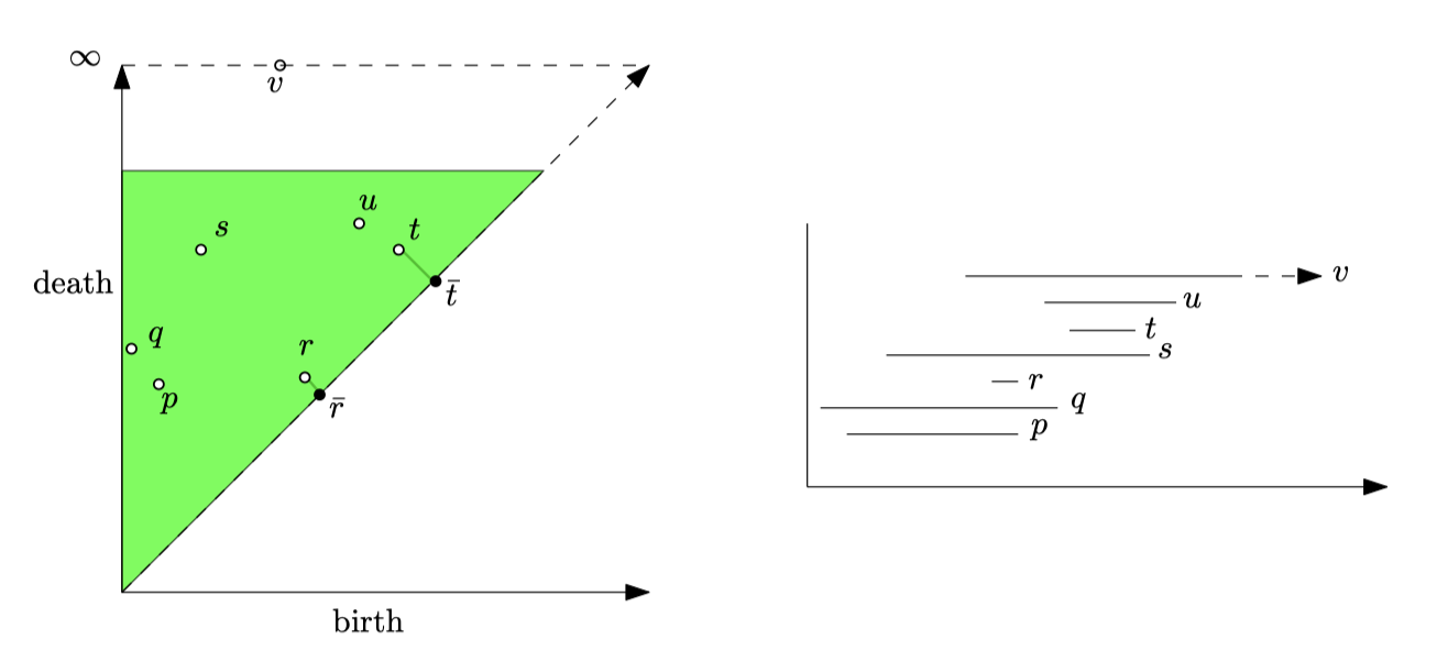
These maps act as a formal “tracking system”. They allow us to define a feature’s lifecycle with mathematical precision: (Zomorodian & Carlsson, 2005)

• Birth: A component is born when it first appears in the filtration and is not yet in the image of a previous map.
• Death: When two components merge as the radius increases, the younger one “dies” by merging into the older, more established one.
• Persistence: The “age” or survival time of the component ($Death - Birth$)

We summarize this lifecycle in a Persistence Diagram ($D_0$). Long-lived features represent real structures (like the main branches of data), while short-lived ones are just noise.

Formalizing the Intuition ($H_0$ Persistence)

If our Hypothesis holds, rare data points are the primary carriers of the manifold’s “skeleton.” While dense regions provide volume, these “topological anchors” define the branching structures that extend into the void.

The importance of such a point is not determined by its density, but by its Topological Impact. We quantify this impact using the Bottleneck Distance, which measures the structural difference between two topological states

Definition

Definition(Bottleneck Distance)

The bottleneck distance $d_b$ measures the minimum cost to match two persistence diagrams. It is the infimum over all bijections $\pi$ of the supremum of the $L_\infty$ distance between matched points:

$d_b(Dgm_p(\mathcal{F}_f), Dgm_p(\mathcal{F}_g)) = \inf_{\pi \in \Pi} \sup_{x \in Dgm_p(\mathcal{F}_f)} \|x - \pi(x)\|_\infty$

Imagine our current labeled dataset $S$ as a set of islands. We build a Vietoris-Rips complex $Rips_{\epsilon}(S)$ by growing balls of radius $\epsilon$ around each point. As $\epsilon$ grows, islands merge. We record the “birth” and “death” of these components in a Persistence Diagram, denoted as $D_0(S)$

The Topological Impact Intuition

Instead of just looking for where the model is “confused” (Uncertainty), we calculates the Topological Impact $\Delta_{topo}$ for any point $x$ relative to a reference set $S$

$\Delta_{topo}(x; S) = d_b(D_0(S), D_0(S \cup \{x\}))$

Points with a high impact are those that create new connected components ($H_0$) or bridge distant parts of the manifold—precisely where rare branching lineages hide. According to the Stability Theorem (Cohen-Steiner et al., 2007), persistence diagrams are stable under perturbations of the underlying function. This means that the $d_b$ we calculate in the impact term is a robust signal that captures real structural changes rather than getting tripped up by random noise.

What does this equation actually mean? The Bottleneck Distance $d_B$ measures the “cost” to transform one persistence diagram into another.

• If $x$ is just another point in a dense cluster, adding it changes nothing structural. The diagrams are nearly identical, so $\Delta_{topo} \approx 0$.
• But if $x$ acts as a bridge between two disconnected components, or extends a rare branch, adding it drastically alters the “death” times of components in the diagram. This results in a large $\Delta_{topo}$.

This gives us a mathematically rigorous way to hunt for “structural change.”

5. Conclusion

This blog formalizes the intuition that in high-dimensional discovery, the most valuable data points are those that fundamentally alter our topological understanding of the system. While the Manifold Hypothesis provides the ideal continuous backdrop for data science, the reality of discrete Point Clouds requires a robust bridge to capture emerging structures.

By utilizing Persistent Homology and the Bottleneck Distance ($d_b$), we move beyond simple density metrics. The proposed hypothesis offers two key theoretical contributions:

• A Sensor for Branching Structures: In complex domains like single-cell biology, rare lineages often appear as sparse “tendrils” extending into the void. Our framework treats these not as outliers to be smoothed away, but as critical changes in $H_0$ persistence—the birth of new connected components that define the manifold’s true skeleton.

• A Mathematical Measure of Discovery: The term $\Delta_{topo}(x; S)$ provides a rigorous way to quantify “surprise.” A high impact score indicates that a point is not just a redundant observation, but a structural bridge or a new direction in the data’s filtration story.

Ultimately, this topological approach suggests that “discovery” is the act of identifying points that force a re-evaluation of the data’s global shape. By focusing on the Topological Impact, we can guide future algorithms to venture into the void, ensuring that the thin, branching structures of rare phenomena are no longer invisible to our models.